
In this article we will explain what a recurrent neural network is and study some recurrent models, including the most popular LSTM model. After the theoretical part we will write a complete simple example of recurrent network in Python 3 using Keras and Tensorflow libraries, which you can use as a playground for your experiments.
Introduction
Before explaining what a recurrent neural network (RNN) is, let's have a quick look at neural networks based on perceptron. Perceptron can predict the output value based on input values. You can think of it as a function of input values, for example, it can tell whether a person is rich depending on the size of his income. But this approach is not suitable for working with sequences. For example, perceptron can't predict the next word in the sentence because if we just feed one previous word on input, there won't be enough information to make a proper prediction. Another example is a prediction of the next value for sine function with a fixed step, based only on the previous value. Recurrent neural network can solve this class of problems by feeding calculations from the previous step to the next step. To do that, RNN has an internal state (also called memory) and we can think of it as a function of input values and the previous state.

You can use recurrent network in different ways. The basic type of usage is to feed input values step-by-step and read outputs for every step. Other ways to use are the following:
-
We can feed a full input sequence and read only the last output;
-
We can skip several first outputs because the network should be prepared before making any predictions;
-
We can feed the output value as an input to the next step. With this approach you can create a network that will be able to generate a new sequence;
-
We can combine two previous ways – feed several input values and then start to feed network's output values as new input values.
BPTT
Backpropagation is used to teach neural networks, but instead of networks based on perceptron, where an error is propagated through layers, in the recurrent networks there is an internal state, so the error should also be propagated through it. There is an approach named Backpropagation Through Time (BPTT), this means that a trained network unfolds in time, so the previous state is replaced with a copy of the network with shared parameters, e.g. f(xt) = f(f(xt-1)).
RNN models
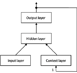
Jordan model
There are several models that use this class of networks. One of the simplest implementations is Jordan model, whose hidden layer is fed not only from the input layer but also from the output layer from the previous time step.
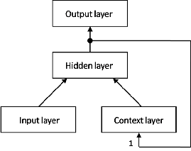
Elman model
Another simple model is Elman model. The main difference is that the hidden layer is fed from itself from the previous step instead of the output layer.
Both models have 2 main problems:
- The first problem is the exploding and vanishing gradient problem. Because of the BPTT usage an error is propagated many times over one element and so it will vanish or explode at the end.
- The second problem is that these networks can't store information from many steps ago.
LSTM
The most popular recurrent network model is Long short-term memory (LSTM). LSTM contains additional elements named 'gates'. These elements make it possible to selectively memorize and forget parts of the sequence.

From left to right an LSTM cell contains:
- Forget gate. This gate is responsible for deciding which part of the previous state should be removed.
- Input gate. This gate is responsible for deciding which part of the input information should be stored.
- Hyperbolic tangent to prepare a candidate to store. The prepared candidate will be multiplied by the result of the input gate. So the prepared candidate can be discarded at all if the input gate will be set to zeros.
- Output gate. This gate is responsible for deciding which part of the calculated state will be sent to the output.
- Hyperbolic tangent is used to normalize the output value.
This structure prevents problems of Jordan and Elmon models because the LSTM cell has forget and input gates, which control how much information should be propagated through the network.
GRU
There are several modifications of the LSTM memory cell and one of them is GRU – Gated recurrent unit. It was introduced in 2014. Instead of three gates in LSTM, GRU has only two gates: reset gate and update gate, so it is a more efficient model.

Main applications of RNN
RNN is mostly used in applications whose predictions depend on the previous context:
- Text translations;
- Speech recognition and generation;
- Handwriting recognition and generation;
- Word prediction for text input smartphones;
- Question-answering and dialog systems;
- Text classifications.
Big companies, such as Google, Apple, Amazon and Microsoft use LSTM in their applications.
Example of prediction on number sequence
We will write a simple example of a recurrent neural network in Python 3 with LSTM cells using Keras and Tensorflow libraries. You can use this example as skeleton for your own experiments. You can get a complete version at github gist.
To run it on your own computer, you need to install the following python packages:
- keras;
- pandas;
- tensorflow;
- matplotlib;
- sklearn.
First we need to create a function to generate our train sequence, in this example we will use a simple sine function:
def seq_func(x):
  return sin(x)
One of the most interesting parts here is the function for network training:
def fit_lstm(train_x, train_y, nb_epoch, neurons):
  x, y = np.array(train_x), np.array(train_y)
  x = x.reshape(len(x), 1, 1)
  model = Sequential()
  model.add(LSTM(neurons, batch_input_shape=(1, 1, 1), stateful=True))
  model.add(Dense(1))
  model.compile(loss='mean_squared_error', optimizer='adam')
  for i in range(nb_epoch):
      model.fit(x, y, epochs=1, batch_size=1, verbose=1, shuffle=False)
      model.reset_states()
  return model
You can see here an LSTM layer. It's important to make it stateful, so the trained state from one input item won't be erased before the next input. By setting 'stateful' to the LSTM layer we get all the responsibility to reset network state in our training. So now we cannot just set epochs number to fit the function. Instead,we call fit and reset_state in a cycle over epochs number manually. Another important thing is to turn off the shuffle in the fit function because the order of the sequence is important for our network.
We need to prepare sequence to train our network:
series = [seq_func(x) for x in range(36)]
supervised = [seq_func(x + 1) for x in range(len(series))]
We will train the network by feeding the elements from the first array and waiting for the elements from the second array as the output. The second array equals to the first, but provides values from one step further.
Call fit_lstm function with series and supervised arrays. We will train our model with 1000 epochs and 16 LSTM memory cells.
lstm_model = fit_lstm(series, supervised, 1000, 16)
After we train our model we can make predictions. We need to feed the model with the initial data to make good predictions.
train_reshaped = np.array(series[:-1]).reshape(len(series)-1, 1, 1)
lstm_model.predict(train_reshaped, batch_size=1)
We will use the last element later, so we aren't feeding it now.
Let's prepare variables to store our predictions so that later we could draw it in the plot.
predictions = []
expectations = []
forecast_result = series[-1]
Next we start making predictions. We can predict values in two ways:
- Predict the next element based on the value of the sine.
- Predict the next element based on the previously predicted value. So our network will generate the sequence by itself.
We will use the second approach in this example.
for i in range(36):
  forecast_result_reshaped = np.array([forecast_result]).reshape(1, 1, 1)
  forecast_result = lstm_model.predict(forecast_result_reshaped)[0, 0]
  predictions.append(forecast_result)
  expected = seq_func(len(series) + i)
  expectations.append(expected)
  print('x=%d, Predicted=%f, Expected=%f' % (len(series) + i, forecast_result, expected))
To show the results more clearly, we will display them on the plot:
pyplot.plot(series + expectations)
pyplot.plot(series + predictions)
pyplot.show()

The blue line is the expected sine function and the orange one is the predictions from our network. The first 36 points are the same as we feed them to network without storing the output. As we can see, our network can generate the sine function by itself.
Conclusion
First, we have explained what a recurrent network is and some RNN models. Next, we wrote a complete simple example of the recurrent neural network that uses the LSTM layer.
You can use recurrent layers in combination with layers of different types, for example with convolutional layers.
You can learn more about LSTM network here. There is the great tutorial about machine learning in general and about LSTM in particular.